F-4E Air-to-Air VI: Assess CATA & Bandit Heading [Essential]

Establishing a Collision Course is reasonably straightforward as long as a lockon is achieved, if the aircraft is equipped with modern avionics, or if the necessary information is provided via a Controller. Things get more challenging if the goal is not alerting the target.

In a no-lockon non-co-speed situation, probably the most common situation, at least in a game, the intercept drift becomes a means of verifying CC. If the drift is minor, a check turn may be enough to correct the geometry. The crew must then monitor the contact moving vertically downwards on the b-scope or towards the centre on a PPI.
Otherwise, the crew must use different techniques.

## CATA approximation
The drift angle, which represents the lateral intercept drift when not on a Collision Course ( θ ), can be used to assess CATA by doubling ρ and turning in the same direction as the drift.

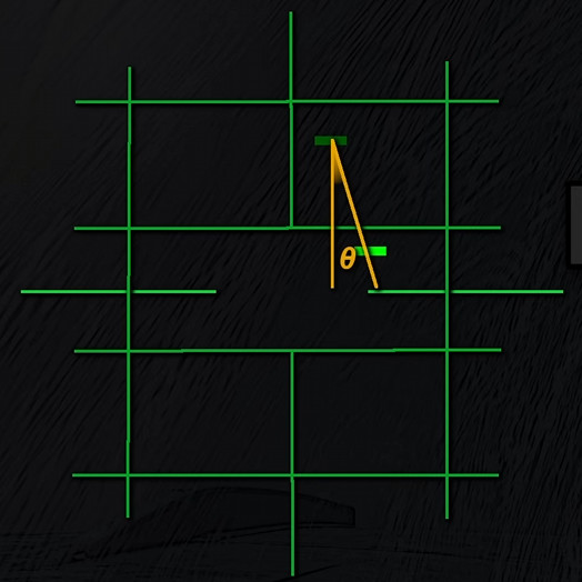
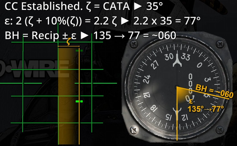
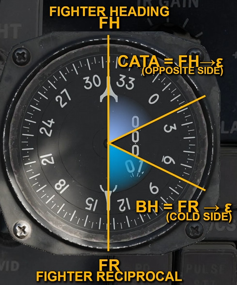
When CATA is established, the target’s heading can be determined using the ATA and the BDHI: the ATA reading on the b-scope, indicated by ζ, is increased by 10% and doubled. The resulting angle ε is computed on the BDHI starting from the fighter’s reciprocal and towards the cold side.

Bandit on the Nose: 0 ATA

A peculiar scenario is the Bandit on the nose.

In this scenario, the reference for the angle determination is not CATA but 0ATA.
Starting with the Bandit’s heading, the drift angle θ is again assessed and doubled. Then, starting from the reciprocal on the BDHI, it is subtracted towards the cold side of the scope and the bandit’s heading is obtained.

The same routine described to calculate the Bandit’s heading at 0ATA is applied to determine the CATA. In the same manner, the drift angle is determined and doubled, and computed using the BDHI to get the desired value. This time, however, the direction is opposite the bandit’s heading.

Note that the previous scenario added 10% to the ζ angle to account for the fighter’s speed advantage.
Here, the 10% increment is missing. I wondered why this was the case because, if taken instantaneously, this computation is valid only in a co-speed scenario. However, if the manoeuvre is considered over time,

Assess drift angle (θ)

At this point of the discussion, a question arises: how can the crew assess θ as precisely and quickly as possible?
Sure enough, one answer is a goniometer, but trying to stick that thing through the VR thingy is not really handy, innit?
Jokes aside, the answer is probably always the same: practice and experience. The cursor can be used as a reference to speed up the learning process.
Note that the bank angle should be zero, otherwise the drift is affected. I used the autopilots in this case, but they can be unreliable.

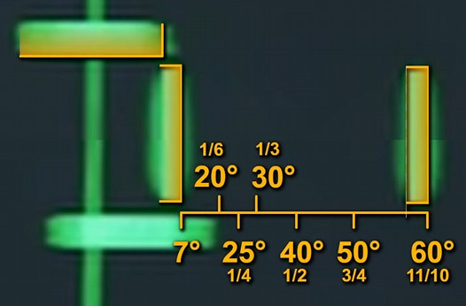
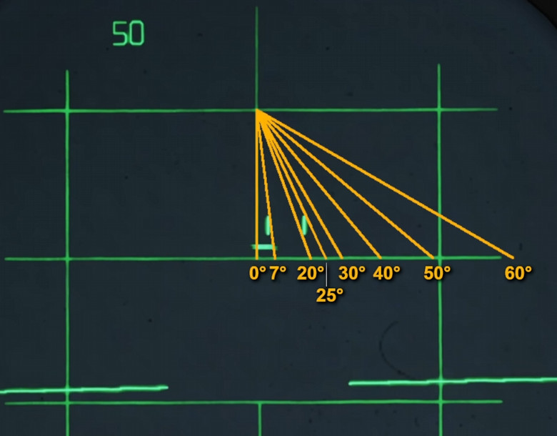
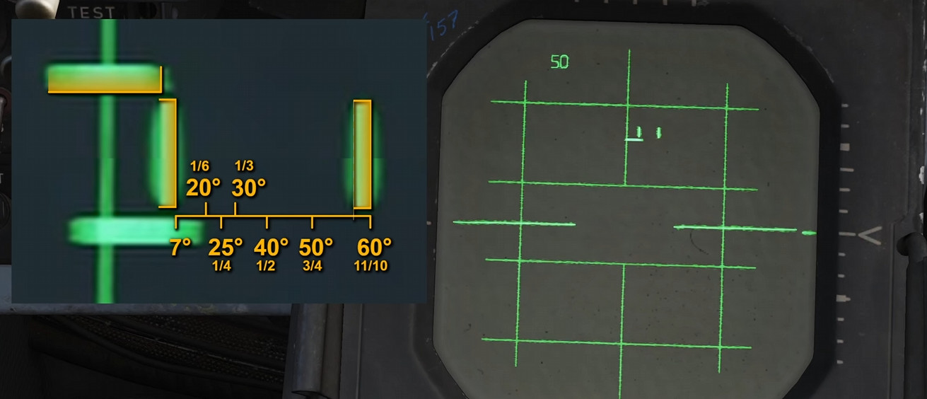
The issue is that a prolonged observation is necessary to assess θ. However, given the properties of the APQ-120, this is not always possible. By comparing the horizontal movement of the return by the time it has moved from slightly above to below the cursor instead, we can assess the desired angle. This is a broad approximation, of course, but it works ok-ish. Later on, experience and guts will tell the crew the size of θ.

Practical Example

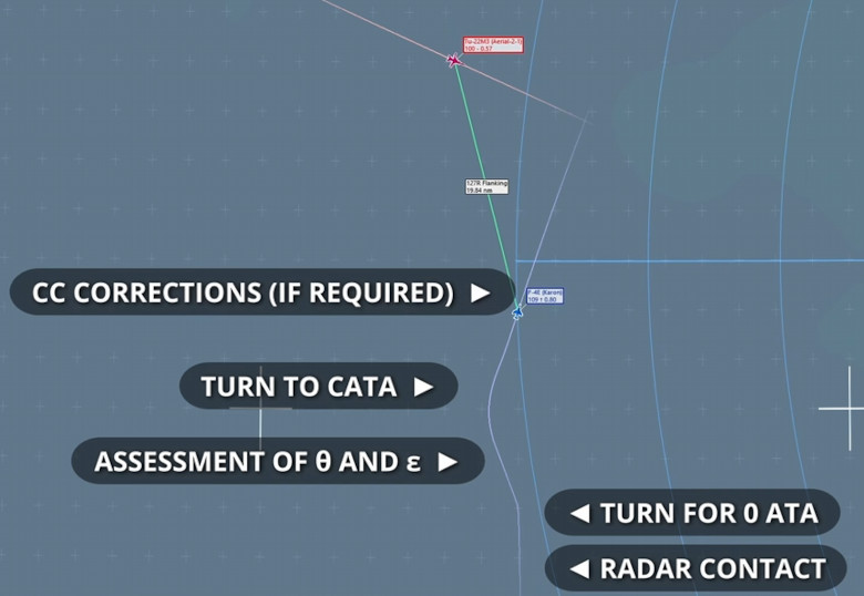
In the scenario represented in the video linked above, a target is spot on the radar at a considerable range. The goal is to assess CATA to reduce the range as fast as possible. This kind of intercept is often concluded with a stern conversion turn, but I maintained the heading for this demonstration.

As usual, we start by assessing the drift, determining the scope sides and then approximating θ.
Θ appears to be slightly less than 20°, therefore ε is circa 40°. The current Fighter Heading is 330, so I turned 010.
The direction depends on the location of the Cold side of the radar scope. In this case, I turned towards the right.

As you can observe in the video, the drift is fundamentally nonexistent. I have been lucky, as such a perfect manoeuvre is hard to achieve, especially when relying only on the autopilots to maintain the heading. As a side note, the aileron trim helps in these cases.

I prefer to show situations with minor errors or imprecisions to demonstrate how they can be mitigated. At the same time, I rarely record more than one take.
If the drift is still present post-turn to the assessed CATA, then a simple check turn should be enough to reduce it considerably. If this is not the case, then either the computation is wrong or the bandit is manoeuvring. In both cases, the crew should take the necessary steps to address the situation.

The beauty of this technique is how quickly it provides an initial reference value for CATA and Bandit’s Heading, which can later be developed as required to reduce the intercept timeline, to set up a VID, a stern conversion for a rear quarter FOX-2, perhaps following a front quarter FOX-1.

Co-speed relations

If speed is known and equal for both aeroplanes, then the intercept triangle becomes a triangle isosceles. In this case, a number of relations become true:

These relations are often described in basic documentation due to their simplicity. Obtaining fundamental parameters such as the Target Aspect just by looking at the scope and noting the Antenna Train Angle is, in fact, quite handy, and serves well ab initio players and pilots alike to get familiar with these fascinating topics.

Observations

The techniques described here are just a fraction of the possible means of determining CATA and the bandit’s heading. As usual, a clever WSO can add all of them to their ever-growing bag of tricks.
The main drawback of the no-lockon procedure is the usage of the drift angle as the main parameter, which can be hard to assess. Co-speed methods are rarely applicable in DCS but can still be used in non-co-speed scenarios. They provide an initial reference that can be refined by further interactions of the same process.

The techniques described in this video are already applicable to a number of procedures discussed already, and will be fundamental in others yet to be covered on FlyAndWire. For example, the “40° cold of CATA” or the “Variable Lag Conversion”.
If you are not convinced yet, consider that a Collision Course is the fastest way to reduce separation. Ergo, a quick means of achieving it, is very valuable.