F-4E Air-to-Air VIII: Variable Lag Pursuit Stern Conversion Intercept

The 1977 “Variable Lag Pursuit Stern Conversion Intercept” technique is based on the approximation of the intercept curve for a 5:4 speed ratio. This wee equation is used to determine a series of parameters, but when you look at it, the standard DCS player’s reaction is “Sir, this is a Wendy Game”.

But, in a curious twist, this method eventually turned out to be simpler than expected, but only once I used the old IT guys’ best friend: flow charts sketched on a piece of paper.

Old and New variables

Before seeing the wonderful flow chart I put together, we must introduce a couple of variables, some old, some new.

• CATA (θ_C) is the familiar Collision Antenna Train Angle. Ergo, the relative bearing (ATA) when a collision course is established.
• R15LAG is a new parameter. It represents the range at which the target is moved from CC to 15° on the cold side of the scope. For the manoeuvre, a 45° AoB turn is usually executed.
• DTG, or Degrees-To-Go, is another familiar concept from the discussion about the intercept geometry, and it represents how many degrees the fighter should turn in order to match the target’s heading. For example, 135 DTG means that the fighter should turn 135° to match the target’s heading. 180 DTG means that the two aeroplanes fly in the opposite direction, ergo the fighter flies following the target’s reciprocal. DTG is referred to in modern times as HCA, acronym for “Heading Crossing Angle.” DTG’s supplementary angle is the “Cut,” a concept used mostly in the US Navy and now considered obsolete.
  This technique uses DTG to monitor and adjust the lag angle as the intercept progresses.

From the mathematical obscenity above, three constants are obtained: 600, 100 and 50. These values are intertwined with range and angles to determine three checkpoints.

1. In primis, R15LAG. The value of this variable is determined as 600 / CATA.
2. Next, the lag angle to nail at 135 DTG, which is obtained as 100 / Range, but with some caveats we will discuss later.
3. Lastly, the lag angle to be matched at 90 DTG. As you can imagine, it is calculated as 50 / Range, but again with some caveats.

Intercept Flow

Since the technique described has a series of peculiarities that can confuse ab initio and veteran players alike, I put together a flow chart to better understand it. I found it to be particularly useful, and I hope you will share the same sentiment.

1. Starting from the beginning of the flow, the crew should manoeuvre to place the bandit on a collision course or flying towards its reciprocal, ergo 180 DTG. I suggest setting up CC as it makes further calculations much quicker. This setup is typically and easily provided by a human GCI. Unfortunately, in-game AI Controllers are not as useful. I described how to assess the necessary parameters in a dedicated article.
2. Whist at it, there are additional parameters to assess, which will be required later. The cold side of the scope is immediate if CC is set up. If not, CATA should be assessed as well. The bandit’s heading instead is immediate if 180 DTG is flown, since it’s the reciprocal value. Once those numbers are known, it is time to enter the thick of the intercept, starting with determining R15LAG.
3. R15LAG can assume three values: less than, greater than or equal to the range between fighter and bandit. Remember that the two aeroplanes are in motion and the range decreases quickly, so try to be on point with your calculations.
   • If R15LAG is smaller than the range, the target should be placed on a collision course and held there until the range and R15LAG match. If you have followed my suggestion initially, you have basically nothing to do besides waiting. Then, follow the next subcase.
     
   • If R15LAG equals range, then the target should be placed at 15° cold and maintained there. Keep in mind that, since no CC is established, the fighter will have to increase its angle of bank to maintain the lag angle.
     
   • Lastly, if R15LAG is greater than the range, the fighter needs room to manoeuvre, and the target should be placed at 45° cold and held there whilst the next oddity is computed. The idea is to anticipate the lag angle at 135 DTG. To do that, we check the range at 180 DTG. During the turn, in fact, the target likely has passed through the 180 DTG. That’s when the range is evaluated and ad hoc action is performed to further hold 45° cold, or place the target to 15° cold. The effect is to have the stick monkey janking the stick all over the place, but this is expected. However, as we will see in the third practical example, if the flow becomes too overwhelming, which is likely when flying without a human pilot or WSO, holding 45° cold until 135 DTG still works, with the caveat that 90 DTG will come up quicker than expected and the overall trajectory will be larger and rounder.
     
4. As the intercept enters the final phase, the cases described before converge. The crew should be proactive and calculate the lag angles at 135 DTG and then 90 DTG.
5. The last step is making sure that the fighter is in the correct position and not too fast or too slow.

If the flow is followed correctly, the manoeuvre should have the fighter rolling out 2 nm behind the target for a speed ratio of 1.12:1, or 5:4. The classic 500 kts vs 400 kts, in other words.

Practical Examples

A series of examples is now presented. The third is the most interesting and complete, but also the one with the highest pace. I recommend checking the previous two before venturing there.
Moreover, the video linked above better conveys the intercept flow.

Example I

The following is my very first successful test applying this technique. There are a couple of errors I will highlight later on. The reasons why the previous attempts did not work are actually interesting. For example, I lost the target in the sidelobes. In this article, I was more proactive and tried to adjust the gain in advance. Another reason is keeping track of everything whilst doing maths and remembering the steps to follow. That’s why I made a dedicated kneeboard page.
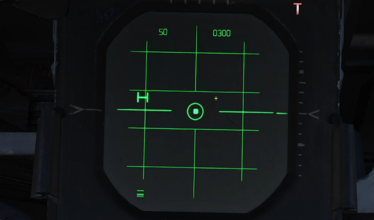
In the scenario running, a collision course is already established, and the target’s heading is 300. Any human GCI can help with that, but DCS is DCS.

Since CC is already established, R15LAG is easy to assess as soon as the target appears on the radar. In this case, CATA is 20R. R15LAG is therefore 30. Following the flow chart, since R15LAG is greater than the range, we hold CC until the range matches R15LAG, and then we turn to place the target at 15° Cold.

Once there, the tricky part starts: guessing the range at which 135 DTG is achieved. Then, apply the appropriate lag angle. DTG is easy to assess: this is nothing new, and we can use the BDHI to monitor it. Since we want to hold the target at 15° cold, the pilot has to input a slight turn, which, in turn, changes the DTG angle.
Once “30”, short for 300°, on the BDHI hits the mark near the label “MAN” is located, we have 135 DTG. That’s when we apply the lag angle. Eyeballing the range and therefore the lag angle takes a bit of experience, but with the kneeboard pages I made, the mental maths component is reduced to a minimum. In this case, it seems that 135 DTG is reached at circa 13 nm, leading to an 8° lag angle. A slight correction is therefore necessary.
Unfortunately, my angles are not precise: lack of experience on the new method, having to monitor the radar, the BDHI, speed and altitude, the APQ-120, and finding the kneeboard data, all require some practice. And, of course, there is a reason why I don’t play as a pilot 🙂
This is even more true as the Phantom II approaches 90 DTG. The range goes down fast, but the lag angle at circa 6 nm is still close to 8° and, in theory, no correction is necessary.
This method is conceived to result in a 2nm rollout behind the target, so, as we approach such a range, V_C should be controlled, and the target placed where necessary. In case of a tanker, for example, we do not want to end up at its 6, but on the dedicated area on its side.

As we have seen, this technique is not that complicated once a bit of visual help is provided. I found it useful to have a flow chart to remind me of the flow and the tables with precalculated R15LAG and the lag angles for 135 and 90 degrees to go.
If you have noticed, I never looked outside the cockpit, which is not something you should do, but I did it purposely to show how this method works in bad weather, low visibility or at night.
The most apparent issue is my inability to maintain the correct lag angle, but it is something that can be offset with some practice. Even so, the method appears to be working quite well.

Example II

The problem with this method, when applied to DCS, is the lack of help from the GCI. I covered techniques to determine CATA and target heading in another article linked above, but they are both based on drift and therefore take time. Moreover, the Variable Lag Pursuit intercept is still based on a 5:4 curve. Different speed ratios may affect the precision of the lag angle tables.

This example shows how the radar can be used to speed up the process of determining CC and target heading via the radar display readouts and the “dot” of the ASE, acronym for “Allowable Steering Circle”. Obviously, this means that a brief radar lock is required, something that creates a number of issues in DCS, given how it is stubbornly fixated on the “stealth factor”.

In this case, I am aware of a contact somewhere in my front quarter at a fairly long range, but no information is provided beforehand. Usually, it is hard to spot such a target, and even the AI GCI can help by providing a BRAA, which is then translated by the crew in ATA. Once the WSO knows where to look, spotting is easy. In this case, instead, I had to monitor the radar “block-by-block” until I noticed a smear not disappearing.
To show something different, let’s use a brief lock-on. Note that this is often suggested by the documentation. By centring the dot and setting the Aspect switch to Tail, the crew immediately obtain CATA and the target’s heading. At least in theory. The dot, in fact, has the tendency to jump everywhere at long range. Personally, I prefer the drift. In fact, if you have noticed, I used the drift to adjust the Phantom’s course slightly and get close to a collision course.

The intercept then continues as usual. Since the range is greater than R15LAG, the collision course is maintained until the two values match at 20nm. At this point, the target is moved to 15° Cold.
Per sé is not complex, but I must highlight again how I lacked precision, as working on controls spread over two cockpits is not immediate.

Example III

The previous examples showed the Phantom intercepting a Tupolev Tu-22, NATO name “Blinder”. Its size made it easy to spot early on the radar. What if, instead, we find a target at a shorter range?
In this scenario, no information is provided directly, but a ground radar is present. Alternatively, the crew can use their Radar Warning Receiver to narrow the search area. In this particular case, I spotted the target via the RWR-extapolated ATA before the GCI provided a BRAA.

The minor drift towards the left revealed the right to be the cold side of the scope. The low drift ratio also indicated that CATA was not far off. I estimated 3°-4°, giving a correction of less than 10°. Next, the heading. A CATA of around 10°-12° means that the target’s heading is approximated as 12*2.1, resulting in circa 23°-25°. The Phantom’s heading is circa 335, leading to an assessed target heading of 360 minus change. To spare my neurons, since I had a lot to monitor already, I rounded to 360.
Now, all this computation required only a few seconds, which is not much, but at a V_C of 800 kts, every second matters. Moreover, these are approximations. I lesson I am struggling to learn is to avoid fixating on the single degree, but be ready to adjust as needed.

At circa 12.5°, R15LAG is 48. The range is quickly approaching 25nm. The solution is to turn hard to place the contact 45° cold and hold until 135 DTG. Crossing 180 DTG, the lag angle to apply at 135 DTG should have been 15° cold. However, I found that, thanks to my tables, I can actually find a more precise lag angle “in real time”, so to speak. I just have to monitor the range.
Unfortunately, I was long on the turn to 45 cold, as I had the feeling the autopilot disconnected, which it didn’t.

Monitoring the closure, I expected the lag angle to be 10° at 135 DTG. The lag angle turned out to be circa 9° but, seriously, this is such a negligible margin…
During the turn, I was close to 90 DTG, and I assumed it to be 8 nm, corresponding to a lag angle of 6°. Therefore, I kept pulling hard. It’s a bit of a shame that I ended up wide earlier whilst manipulating the radar and the autopilots, otherwise the turn would have much more precise.
Something I did not do, and on purpose, is verify V_C. As TacView showed, rather than being a 5:4 speed ratio, ergo a 1.25:1, this intercept was actually a quite absurd 1.65:1. If the goal is to saddle or at least avoid overshooting, the throttle should be managed more carefully.

It is worth mentioning that the actual procedure involves even more dramatic manoeuvres than what I showed. In particular, once the 180 DTG computation is satisfied, action should be taken immediately to hold the target at 45° cold, or to hard turn in the opposite direction to have it at 15°. Since I was flying on my own, that was a bit too much to manage at such a high V_C, so I opted for the easier solution, which is holding 45°. The drawback is that a harder counterturn is required, and 90 DTG comes up very quickly.

Final Notes

To wrap this technique up, here are a couple of final notes and considerations.

• Rollout
  As demonstrated, this technique is quite straightforward once understood. It is also easy to adjust to different requirements. For instance, different rollout distances. The discussion so far had, in fact, the objective of performing a 2nm rollout behind the target. If shorter or wider distances are required instead, all the crew has to do is manipulate the constants. For example, if the goal is 1 nm rollout, then the constants should be halved. Vice versa, for a 4 nm rollout, they should be doubled.
• Altitude
  To keep things easy, I set up every scenario to be co-altitude. In reality, you may want to have a negative offset. Do not be afraid to reduce altitude: it makes the target more visible and yours harder to spot, assuming they are flying a properly made module. Obviously, the drawback is the necessity of updating the antenna elevation angle as necessary.
• Improve situation assessment
  In case no information is provided and you cannot or do not want to rely on your guts and experience to eyeball data, you can put the target on the nose. The 0 ATA situation simplifies several calculations and can be beneficial to ab initio players, especially.