
The Detail Data Display
Most of the introductory details about the DDD are covered in the manual, so I will not repeat them here. Just to recap, the DDD displays different measures depending on the radar mode or the function used (i.e. Pulse, AN/APX-76 and Pulse Doppler).
The DDD in Pulse mode has been mentioned several times already: it is a b-scope, showing Azimuth as the abscissa, and range as the ordinate. This mode is really handy for intercepts and angle considerations as it is basically a top-down view clearly showing a potential drift.
The DDD in Pulse Doppler mode shows the Azimuth as the abscissa, but the closing rate but versus the ground, rather than the F-14. What does it mean?
As mentioned, PD mode removes the F-14 as a factor in terms of speed. Understanding how this works is fundamental, as the TID in Aircraft Stabilized mode does not provide all the information the RIO may need or want at a glance. Not to mention when the target is beyond “RWS-range”, and PD SRCH is the only radar mode providing data.
Happy 3+ Friends
The DDD does not provide a variety of information as the TID does. Contrary to this device, in fact, it cannot show different values or information on demand. Therefore, if the RIO is limited to the DDD by malfunctions or radar (i.e. contacts are displayed only in PD SRCH), combining the DDD with other devices can drastically augment the SA. This is also a good practice to better understand the situation at a glance, without cycling through the TID readouts by means of the CAP.
For example, noting which bar returns a contact can help to assess if a contact is higher or lower than the F-14, and if the situation changes over time. Of course, due to the range, even 1B is very tall, but it is still a good indication (you can use my Antenna Elevation model “backwards” to get ΔALT from range and angle). Speaking of range, an empirical and rough way to determine it is switching from PD SRCH to RWS. If the target is shows in PD SRCH but not in RWS, then it may be further away than a certain range, depending on the aircraft. This last information can be sometimes obtained by means of the RWR if the target is a fighter.
DDD in Pulse Doppler mode
When a Pulse Doppler radar mode is selected, the display switches the Range on the ordinate with the Relative closure, maintaining the Azimuth on the abscissa.
This mode is less intuitive than Pulse, but it greatly complements the TID in Aircraft Stabilized mode, providing the RIO with the information that the TID does not immediately show.
The Aspect Switch
Recently implemented, the Aspect switch not only affects how the DDD presents information, but also affects directly how the radar operates:
“In the pulse doppler search modes it controls the rate processing windows of the radar, NOSE sets 600 knots opening to 1,800 knots closing, BEAM sets 1,200 knots closing to 1,200 knots opening and TAIL sets 1,800 knots opening to 600 knots closing.”
The effect on the DDD is simple: the central mark on the left side in “Beam” represents 0 kts. The marks above and below indicate either +600 kts or -600 kts. If “Nose” or “Tail” are selected, the scale is moved a notch above or below, but the interval between each mark is always 600 kts.
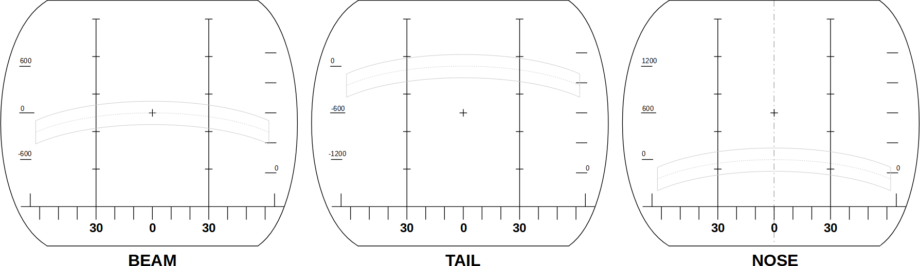
Mainlobe clutter trace
When the Mainlobe Clutter filter switch is used to turn the homonymous Filter off, ground returns are not removed any more, and they can appear on the DDD.
This is how the Aspect switch affects where the trace is displayed:

In very simple terms, the MLC trace shows where the relative speed is zero, so it normally “follows the zero around” as the switch is operated.
ZDF: Is it Curved or is it Flat?
The MLC trace is not flat, and the reason is immediate. What about the area filtered by the Zero Doppler filter?
Since the ZDF “surrounds” VF14 and is not related to the contact per sé, it is always positioned at -VF14 ± 100 kts. Unfortunately, this means that the ZD filtered area fluctuates following the speed of the fighter. The RIO should be always aware of the speed of the F-14, to immediately understand what happens if a target suddenly disappears from the scope.
The following video tries to visualize the effects of the ZDF on the DDD by showing multiple aircraft, either flying true or parallel stern, that appear and disappear due to the effect of the Zero Doppler Filter.
The dummies start at a speed of 250 kts, whereas the F-14 starts at 450 kts. The contacts then accelerate to 650 kts and then slow down again to 250 kts. Therefore, the targets spawn at 200 closing, reach 200 opening, and then slow down again, passing the ZDF twice in the process.
Two properties are worth noting:
- the area on the DDD where the contacts fade: as mentioned, it is flat;
- drift: pay attention to how the targets drift as the speed changes. The angles affect the relative speed, and consequently what is filtered by the ZDF.
Using the Detail Data Display in Pulse Doppler Mode
In Search mode or, better, in non-STT modes, the DDD complements the TID providing additional information. This is especially true in the case of the Aircraft stabilized mode.
Since the vector displayed in such mode is the subtraction of the velocity vectors, it does not change depending on the position of the target. Moreover, due to how the track is calculated, it is sometimes hard to spot changes in heading or speed, which immediately affect the closure rate and are giveaways (especially the heading) of a target trying to defend, either preventively or actively.
In Ground Stabilized mode, when the NAVGRID is on the aircraft is patrolling and building or maintaining Situational Awareness, the DDD provides information that Range While Search does not provide, since this mode does not build any track (not mention when the contacts are so far away that PD SRCH is the only meaningful mode).
Displaying the relative closure rate, it can provide some details useful to the RIO to better understand the situation. For example, a non-drifting target (although the drift is harder to appreciate in PD than P mode), with high closure may indicate that a bogey placed us on collision course, and it is intercepting us. Similarly, if the relative closure drops, it may indicate that the target is manoeuvring (perhaps a CAP now turning cold).
Another fundamental feature is the ability to understand when a target is about to notch or if it is trying to hide in the ZDF area. These details are not available directly to a RIO that relies only on the TID AS (at least not in such as direct way as by means of the DDD).
A Potential Drawback: Clutter
Who doesn’t love some Maths?
Welcome again to the best part of any article: Trigonometry (aka the proof that High School is useful)!
The Closure Rate, VC has been recently discussed in this simple article. Make sure you checked it before proceeding.
The formula I used to determine the Closure rate in the simple scenarios about to be discussed (all co-altitude) is the following:
As mentioned, the DDD does not display VC on the ordinate, but the Relative Closure (it does display a mark on the right side). This is explained in the manual:
“[…] the radar itself only reads relative airspeed which is then modified by subtracting own airspeed for display on the DDD.”
This means that the displayed contact will have a relative rate equal to:
This equation allows the RIO to understand the displayed values.
Thoughts: An Alternative Implementation?
I have a question. What happens if, rather than subtracting VF14, it is set to zero?
If VF14 = 0, then its component in the VC equation becomes zero, but the ordinate on the DDD becomes even more representative of the aspect of the contact. In fact, when the ordinate equals the speed of the target, then the Target Aspect is zero: that would be a neat and almost instantaneous way to determine the target aspect!
Instead, the implementation of the DDD is a VC – VF14 so, although the ordinate is still indicative of the aspect of the contact, it is… well, not as cool.
(unless I’m missing something, which is entirely possible).
Setting VF14 to zero:
VREL = – VTGT * cos (BRG – HDGTGT)
It appears even more immediate now how, if the target is Hot, the BRG matches the Bandit reciprocal, the VREL tends to be closer to the speed of the target.
In fact:
(The sign does not matter)
Therefore:
VREL = 0 * VF14 * cos (BRG – HDGF14) – VTGT * -1 = VTGT
Example
HDGTGT = 205°
BRG = 025°
We can determine the TA as usual:
BR = 025°
TA = BR → BB = 025 → 025 = 0°
Now, proving the equation:
VREL = – VTGT * cos (BRG – HDGTGT) = – VTGT * cos (025 – 205) = – VTGT * -1 = VTGT
The implementation we have in the DDD better represents the positioning of the target (see the examples discussed below and the video above), but having a quick way to discern the TA would be neat. What do you think? (or, What am I missing?)
UPDATE 03/03/2023
Looking back, this was an interesting idea, but the actual implementation is vastly superior as it allows seeing both MLC and ZDF better in any condition, and possibly something else I am not aware of yet.
I’m leaving this part here because, albeit useless, it proves again how first impressions and initial thoughts are often plagued by ignorance, and learning is a long and never-ending process.
Practical Examples and Empirical Demonstration
The following scenarios aim to better give some ideas about how the DDD can be used and which are some of the information provided. At the moment, the DDD does not provide all the information displayed on the manual (such as the AGC Trace).
Each scenario sees a contact on the nose (FH = BR) and a second contact, with the same speed and heading, but with an offset on the azimuth.
I also approximated the Notch gate (±133 kts around V0 and the Zero Doppler Filter ±100 kts). Moreover, I added the representation of the vector as it is calculated in the TID in Aircraft Stabilized mode. In these scenarios, the “height” of the vector, when the speed of the F-14 is not considered, matches the VREL value.
I included empirical evaluations to confirm that the representation of the theoretical outcome is, in fact, correct. However, that replicating the exact scenarios in DCS is very hard, so there are some discrepancies.
Scenario I

The scenario above, replicated in DCS, looks like the following:

By measuring the distance between different points, using the known 600 kts mark as meter, we can determine the speed-value of the other contact. The results are, all things considered, fairly similar:
The contact already matches the 600 kts mark.
ATA = 45
45.5 : 600 = 19.2 : x
→ x = 253.2 kts
Considering the many imprecisions introduced by this empirical approach, such as the difficulty in creating a proper scenario in DCS in terms of angles, or even nailing the correct ATA considering how fast the aircraft are moving and the consequent drift, the result is quite convincing.
Scenario II

The following is the same scenario in DCS:
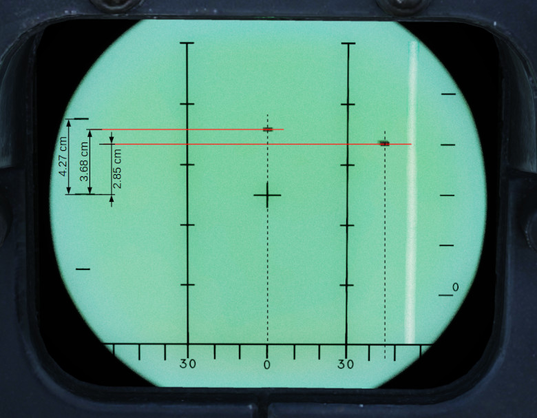
Same process as before to determine VREL empirically:
ATA = 0
36.8 mm → 517 kts
ATA = 45
28.5 mm → 400 kts
The resulting value is still quite similar. Note that the value in cm is different due to the zoom level I was using at that moment and how the screenshot was adapted to LibreOffice Draw.
Scenario III
A different example here: both notching and ZDF.

The in-game scenario is a bit different. In fact, none of the returns are visible immediately.
On the left, the target appears almost immediately, as soon as the closure drops under -133 kts (I did not nail the correct ATA, btw).
On the right, the target is hidden in the ZDF, and it appears much later compared to the previous.

Let’s check the numbers:
Notching Target (Left)
10.9 mm → -144 kts (negative, as the target is opening)
ZDF (Right)
53.4 mm → -705 kts
This scenario is different, since no contacts were immediately visible. However, the returns on the DDD appear at values that match our expectations: in other words, the first values right after the intervals affected by the filters.
Try it Yourself!
The mission, with all the scenarios covered in this article, is available here. Keep in mind it is not perfect and the angles are eyeballed, but it should give you a ready-to-go scenario to play with the DDD.
I hope you have found this article interesting. Feel free to leave a comment, feedback is always welcomed!
I plan to put together another “snippet” video about the DDD as soon as I have some spare time.